


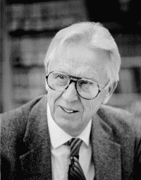
 Father
of Satellite Meteorology
Father
of Satellite Meteorology
Dr. Verner Suomi |
Adapted with permission from an original text by Russell Hall, Editor, UW-Madison Space Science and Engineering Center
Introduction
This lesson features Dr. Verner Suomi, telling the story of why he became known as the Father of Satellite Meteorology. Student activities include hands-on learning about satellites, applying knowledge of satellite imagery, and understanding more about occupational jargon.
Focus Questions
How did Dr. Verner Suomi influence the field of satellite meteorology?
What are the different types of satellites that meteorologists use for collecting weather data?
How do you interpret satellite imagery?
What is the occupational jargon related to meteorology?
Learning Objectives
To appriciate the contributions to weather science made by Dr. Verner Suomi.
To identify the different types of weather satellites and their uses.
To understand that every occupational and special interest group has
its own specialized language or jargon.
Preparing to Teach this Lesson
Read this story of Dr. Verner Suomi's development of weather satellites. Print and copy it for your students to read. Print and make overheads of the three satellite images below. Gather and prepare the materials needed for students to make satellite models in the Build Your Own! activity.
The Father of Satellite Meteorology, Verner Suomi
"You've certainly gotten a lot of mileage out of freshman physics."
According to Dr. Vernor Suomi, this was a comment he heard more than once during his career, and he was proud of it. With his unique combination of determination, hard work, inspiration--and those freshman physics--Dr. Suomi became known internationally as the "Father of Satellite Meteorology." His research and inventions have radically improved forecasting and our understanding of global weather.
Dr. Suomi grew up in Minnesota. He wanted to be an engineer, but couldn't afford to pursue an engineering degree at a university. Instead, he attended a teachers' college and taught high school science for several years. When World War II began, he enrolled in a Civil Air Patrol class. Members of Civil Air Patrol were civilian pilots and aviators who flew civilian aircrafts to assist the United States government during the war. It was through this class that Dr. Suomi first became acquainted with the field of meteorology.
This new love led him to the University of Chicago where he continued his meteorology studies and trained air cadets in basic forecasting. In 1948 he became one of the first faculty members in the University of Wisconsin-Madison's newly created Department of Meteorology.
During his first years at UW, Dr. Suomi continued to pursue his Ph.D. at the University of Chicago. For his doctoral thesis, he measured the heat budget of a cornfield. Dr. Suomi himself admitted this was not the most exciting work, but the project led him to think about Earth's heat budget. The obvious way to measure this was to use satellites, which by the mid-1950s were emerging as a meteorological tool.
"When I began my work with meteorological satellites," Dr. Suomi said,"no one in the Department of Meteorology seemed particularly interested. But they didn't try to impede progress in the field, for which I'm forever grateful."
There are two main orbits, or paths, which weather satellites take around Earth. The earliest satellites followed a Low Earth Orbit (LEO). Satellites in this orbit fly at an altitude of approximately 850 km. Although there are many orbit paths a LEO satellite may take, the most common orbit is one that circles the Earth from pole to pole. They are therefore known as polar-orbiting Earth satellites (POES). Polar-orbiting satellites are able to view all regions of Earth in only one day. For this reason, they are very useful in studying global weather patterns. The National Oceanic and Atmospheric Administration (NOAA) currently has two polar-orbiting satellites in operation. One views regions of the United States at 2 p.m. and 2 a.m. local time, while the other views them at 10 p.m. and 10 a.m. local time.
In 1959, a Low Earth Orbit satellite went into orbit, carrying with it a flat plate radiometer of Dr. Suomi's design. This device measured Earth's heat budget. Combining this with weather balloon data on atmospheric cooling, Dr. Suomi was able to demonstrate the important role that clouds play in absorbing radiated solar energy. These studies set the stage for the full-scale integration of satellites into the field of meteorology.
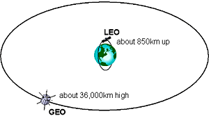
LEO and GEO orbit elevations
The other type of satellite follows a Geostationary Earth Orbit (GEO), in which the satellite flies at the same speed as Earth's rotation. The first of these was launched in 1966. This satellite, orbiting approximately 36,000 km above Earth's equator, appears to be fixed in one location. Instruments on geostationary satellites have a constant view of the mid-latitudes and the tropics, but a very limited view of the poles.
Geostationary satellites are largely used to track the movement of weather systems. If you tune into the daily weather forecast on television you will surely see satellite images of a weather system's movement. Currently, the United States has two geostationary satellites in operation by NOAA. One has a view of the West Coast region and the other has a view of the East Coast region.
Dr. Suomi understood the potential benefits of observing a single weather phenomenon at frequent intervals, but in 1963 geostationary satellites did not exist. When he read about NASA's plan for a Geostationary Earth Satellite, he suddenly realized that placing instruments capable of recording data related to earth's atmosphere and surface onboard such a satellite would open new doors for meteorological observation. As Dr. Suomi said, "The weather moves, not the satellite." Thus, it would be possible to observe weather patterns' development, a study certain to improve weather forecasting and further the field of weather science.
In 1965, Dr. Suomi and Robert Parent, an electrical engineering professor at UW-Madison, founded the Space Science and Engineering Center with funding from NASA and the National Science Foundation. SSEC was destined to become a hotbed of invention and research. Drs. Suomi and Parent continued to pursue the expanding possibilities of geostationary satellites. Dr. Suomi's realization of his idea for gathering meteorological data from geostationary satellites was SSEC's first great invention. He called it a spin-scan camera.
Dr. Suomi's spin-scan camera instrument is not actually a camera. It is composed of two types of radiometers. One type measures the amount of visible light from the sun that is reflected by Earth's surface or clouds. The other type measures the amount of radiation emitted by these sources. One can see how Dr. Suomi's original work with cornfield heat budgets influenced his thinking, but the shift in scale is staggering.
The premise of the satellite dictated the "spin-scan" name. The satellite spun in its orbit, in the same way that earth rotates while at the same time orbiting the sun. The camera shifted slightly with each rotation, scanning small strips of earth. These strips could be combined into a global weather picture in thirty minutes.
Professors Suomi and Parent saw their spin-scan camera launched in 1966, on board the Geostationary Advanced Technology Satellite 1. It is no exaggeration to say the spin-scan camera revolutionized satellite meteorology. Now it was possible to measure and track air motion, cloud heights, rainfall, even pollution and natural disasters. This technology soon became an operational necessity. The improvement in forecasting meant thousands of lives saved during severe weather events.
Dr. Suomi, along with engineers and scientists at SSEC, continued working with his original spin-scan idea. By 1967 the spin-scan pictures were in color and by 1971 SSEC scientists and engineers had begun work on an instrument capable of profiling the atmosphere's temperature and water vapor from geostationary satellites.
Meteorologists were now looking at three types of satellite images: visible, infrared and water vapor imageries. Visible images are obtained from data collected by radiometers that measure visible light being reflected off Earth's surface or by clouds. Regions that reflect little visible light will show up darker than regions that reflect a lot of light. For example, regions that are experiencing nighttime will be completely dark. In addition, bodies of water reflect less light than land. Therefore, lakes and oceans will appear darker in visible images than will land masses. Clouds and snow tend to reflect a lot of light and will appear much whiter than everything else.
Infrared images are obtained from data collected by radiometers that measure the amount of radiation emitted by Earth's surface or clouds. This radiation is then converted into a temperature.In infrared images cold surfaces are white while warm surfaces are black. With respect to clouds, those that are at a higher altitude will have a lower temperature, and thus appear whiter. On the other hand, low-level clouds will have a warmer temperature, thus appearing darker. Since all objects emit radiation all of the time, infrared images can be taken without the presence of sunlight.
Water vapor images are obtained from radiometers that measure the amount of radiation emitted by water vapor in the atmosphere. These data are collected from the middle and upper troposphere. Regions of low relative humidity (dry regions) are characterized by black and dark grays, while regions of high relative humidity (moist regions) show up as lighter grays.
By 1970, the flow of meteorological data had become a flood. To make sense of this data, or, as he put it, "to get a drink from a fire hydrant," Dr. Suomi became the driving force behind the development of a computer system to gather and handle the wealth of data and images.
Like many of his ideas, Dr. Suomi's solution was rooted in freshman physics, his observant nature, and the inspiration he drew from his everyday life and work. The Man-computer Iteractive Data Access System (McIDAS) sprang from an idea he had while watching football on television. Just as TV viewers wanted important plays slowed down and replayed, he realized what he really wanted was an "instant replay of satellite pictures." He wanted to slow them down, replay them, and have a computer analyze them.
SSEC engineers and programmers had the skill to bring Professor Suomi's idea to life. In 1972, at the age of sixty-six, Dr. Suomi introduced McIDAS to the world. Today, McIDAS is in use by the National Storm Prediction Center, the National Weather Service, the National Transportation Safety Board, and NASA Goddard Space Flight Center. Many other government agencies and private companies rely on McIDAS as well, including meteorological centers in Spain, Australia and Japan.
Dr. Suomi's creative impact did not end there. He paved the way for data-collecting missions to Venus, Jupiter, Saturn, Uranus and Neptune, leading to better understanding of their atmospheres. He continued to teach at the University of Wisconsin until his retirement from teaching in 1986. He retired from the SSEC directorship in 1988, but stayed active in research by designing instruments, directing field experiments, and advising scientists in atmospheric science projects until the week of his death in July 1995.
Suggested Activities
Occupational Jargon
One aspect of occupational folklore is jargon, the specialized talk shared by members of a cultural group. The people who share the common activity also share the words to describe what they do. Many weather terms we take for granted today were originally weather worker jargon. For Dr. Suomi's part, many words we hear on TV news weather reports stem directly from his work with the spin-scan camera. When most people hear the term "front" in relation to weather, they know what it means. But if it weren't for the high altitude weather observations Dr. Suomi pioneered, that might not be the case.
To help students understand that jargon is the technical vocabulary for an occupation or pastime, have them examine the specialized terms used by the following groups: taxi cab drivers with Union Cab Company in Madison, Taxi Speak; Great Lakes sailors' shipping terms, Shipping Glossary; computer hackers, The Jargon File; gardeners, Garden Jargon Made Easy; military lawyers, Military Jargon; and even teachers, Glossary of Educational Terms.
Assign students to watch the weather forecast on the evening news. Have them write down weather words they know the meaning of and those they don't. Make a list as a class and define them together, and use this as a lead-in to a discussion of satellite meteorology. Identify these terms as meteorology jargon.
Have your students ask their family members about jargon they use on the job. Each student can write a short essay on a family member's work, including what they do, what jargon goes along with it, and what the terms mean.
Working as a Team
Teamwork is an important part of workplace culture. As your students have read, the scientists who worked with Dr. Suomi played a crucial role in bringing his ideas to life. Ask your class some brain-starter questions about teamwork. What does it take to be part of a team? What are some of the things teams can do that one person alone might not be able to? Now have them write a short response on a time when they were part of a team or group. Ask them to include their role, how it was important, and what some of the other people's roles on the team were.
Which Type of Satellite?
Have students watch the weather report on their local news channel for one week. Each time they see a satellite image or loop being used by the meteorologist, have them briefly describe the weather features shown. Was a GEO or LEO satellite used? How can you tell? What other weather features could be studied by satellite images/loops? Why would these images/loops be useful for a meteorologist?
Discuss these questions with your students:
What type of satellite is used to track large-scale weather systems? What type of satellite is better for viewing small-scale features on the Earth over a single country? Besides weather, what else could be beneficial for satellites to observe? Would it be best to use a LEO or a GEO satellite? Why?
Satellite Images
Have students study the images below. Which one is an infrared satellite image? Which one is a visible satellite image? Which one is a water vapor image? Explain.
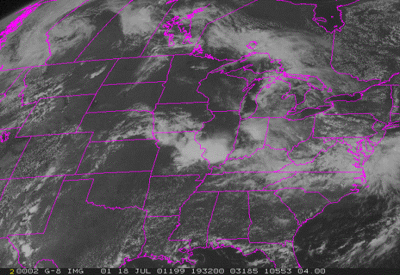
Figure 1. A visible image, taken from a GEO satellite, of the weather over a region of the continental United States and southern Canada on July 18, 2001.
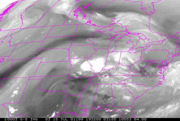
Figure 2. A water vapor image, taken from a GEO satellite, of the weather over a region of the continental United States and southern Canada on July 18, 2001. Compare this image to the visible image above.
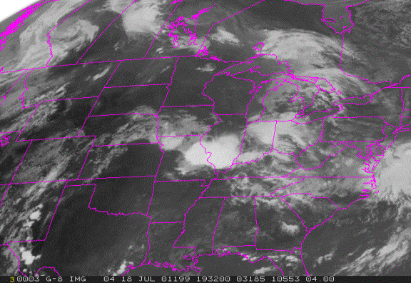
Figure 3. An infrared image, taken from a GEO satellite, of the weather over a region of the continental United States and southern Canada on July 18, 2001. Compare this image to the visible and water vapor images above.
Build Your Own!
Have students construct models of Earth and the two types of weather satellites. The supplies that will be needed are: a sheet of light cardboard or one side of a manila folder, 6 straight pins, tape, a pair of scissors, a pen or fine marker, 2 paper clips, photocopies of the polar-orbit and geostationary-orbit templates, and 2 styrofoam balls, each 3 inches in diameter. Have your students follow the directions below.
General Preparation:
- Using the orbit templates as a guide, cut out one ring representing a polar orbit and one ring representing a geostationary orbit. (Hint: You'll find it easier to cut out the inside circle if you fold each paper ring in half before you begin).
- Lay the two paper rings on one side of a manila folder or sheet of light cardboard. Trace the outlines, and cut out the two orbit rings.
- Glue each paper ring onto a cardboard ring so the rings are rigid.
Making the Polar-Orbiter Model:
- Stick one straight pin into a Styrofoam ball. Stick another pin in the other side of the ball, directly below the first one. Label the points "N" and "S" for the North Pole and South Pole.
- Use a marker to draw a circle around the ball from pole to pole.
- Place a polar-orbit ring over the ball, lining it up with the circle you just drew.
- Tape an orbit ring to the pins at the poles. The ball should rotate freely under the ring, as shown in the illustration on the template.
- Clip one of the satellite rings to the polar orbit at the zero mark on the orbit, halfway between the North Pole and South Pole. This (the equator) will be the starting point for the satellite-path demonstration to follow.
- Holding the model by its orbit, rotate the Earth to the right until it lines up with the line you drew for the polar orbit.
- Move the satellite northward until it is over the North Pole.
- Continue moving the satellite in its orbit until you reach Earth's equator again. Remember, as the satellite moves, Earth turns slightly on its axis. Rotate the Earth a little to the right.
- Move the satellite further until it is now over the South Pole. Also, rotate Earth just a little more on its axis.
- Again, continue moving the satellite until it reaches the equator. Rotate the Earth to the right a little bit more.
- Repeat steps 7-10 until you've made a complete circle around the Earth. How many times did the satellite cross the equator?
Making the Geostationary-Orbiter Model:
- Take the remaining Styrofoam ball, and draw a circle half-way between the poles. This line will represent the equator.
- Place two pins opposite each other at the equator.
- Use a marker to draw another circle around the ball, this time from pole to pole. Stick two pins into the line, one opposite the other. Label the points "N" and "S" for the North Pole and South Pole.
- Line up the zero mark on the orbit with the equator, as shown in the small illustration on the template. Tape the geostationary-orbit ring to the pins. The ball should rotate freely under the ring, as shown in the illustration on the template.
- Clip the satellite on its orbit at the zero mark, halfway between the North Pole and South Pole. This will be the starting point for the satellite-path demonstration to follow.
- Hold the Styrofoam ball by the pins at its poles, and rotate it slowly to the right. Will the satellite ever be able to photograph the other side of the Earth?
Further Resources
The Verner Suomi Virtual Museum developed by the Cooperative Institute for Meteorological Satellite Studies, goes into greater depth on most of the topics covered above, including Dr. Suomi's career, satellites and interpreting satellite imagery
Satellite Meteorology for Grades 7-12 is an on-line course developed for middle and high school science classes by the Cooperative Institute for Meteorological Satellite Studies at UW-Madison.
Learn more about the Civil Air Patrol. an organization that launched Dr. Suomi's career in meteorology.
This Iron County Cultural History and Art Lesson features English Language Arts lessons on the jargon of loggers and miners in Michigan's Upper Peninsula. This lesson from NASA features Medical Jargon as a way to understand the Latin root of many technical terms.
Standards and Benchmarks
| Grade 4 | Grade 8 | Grade 12 | |
|---|---|---|---|
| Language Arts | A.4.1; A.4.2; A.4.3, A.4.4; B.4.1; C.4.2; D.4.2; E.4.1 | D.8.2 A.8.1; A.8.3; A.8.4; B.8.1; E.8.1 | A.12.1; A.12.2; A.12.4; A.12.11; B.12.1; C.12.2; D.12.2; E.12.1 |
| Social Studies | A.4.1; A.4.2; A.4.7; B.4.1; B.4.8; B.4.7 | A.8.1; A.8.3; A.8.7; A.8.8; B.8.1; B.8.8 | B.12.8, B.12.9 |
| Science | B.4.2 | B.8.2 | B.12.1, B.12.2 |
| Business | J.4.7; J.4.8; K.4.4; K.4.5 | J.8.10; K.8.9 |

